Neuron training
Bob can say what power he wants. He does not supply the box’s weight or bias. The box must use the gap between its prediction and Bob’s answer to move its adjustable numbers.
AFTER THIS LESSON By the end, you can tell a human-provided target from a learned parameter, measure one mistake, and calculate one training step.
Training examples
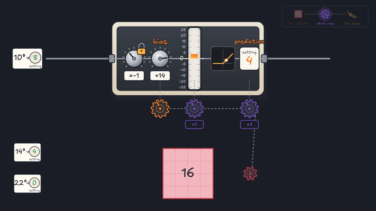
So far, we typed the neuron’s numbers ourselves. To let it learn, Bob supplies examples instead: a room temperature and the heater power he wanted there. For this first training step, the room is 10°C and Bob’s target is 8 power. We hold the weight at −1 and let only the bias move. Its starting value, 14, is a guess, not a number Bob taught the machine.
With that guess, the neuron says 4. It is 4 short of the target. We turn the gap into one nonnegative score by squaring it: 4 × 4 = 16. This score is the loss. A perfect answer has loss zero. Here we use a single example so every number stays visible; a full training run measures many examples.
From a wrong guess to a smaller loss
−1 × 10 + 14 = 4; (4 − 8)² = 16loss 16rate of loss at bias 14 = −8raise bias14 − 0.25 × (−8) = 16new bias 16−1 × 10 + 16 = 6; (6 − 8)² = 4loss 4Gradient direction
Near bias 14, raising the bias by a tiny amount raises the prediction too. That makes the gap smaller, so the squared loss falls. The local rate of change is −8: increasing the bias by a little lowers loss by roughly eight times that little amount. The backward calculation that finds this rate is called backpropagation. Moving the bias opposite the rate is gradient descent.
The rate tells us which way and how strongly the loss changes nearby; the learning rate decides how far to step. Try 0.25 first, then compare with 1. A huge step can leap past the best bias and leave the loss just as large. One example also cannot tell us whether changing the weight or the bias is the better general rule. More examples expose that difference.
Try an update
The example stays fixed: 10°C, desired power 8. Change the step size to see how learning behaves.
The prediction is 4 short. A higher bias would reduce the mistake.
Predict before you reveal: what happens with the huge learning rate of 1?
The first rate is −8, so bias 14 jumps to 22. The neuron then predicts 12 instead of 8; the gap is 4 again and loss is 16. It landed on the other side of the best bias, which is 18 for this one fixed example.
WHAT CHANGED? The example supplied a desired output; the calculated rate told the bias how to move.
Key concepts
- Training example
- An input paired with a desired output supplied from outside the model: here 10°C paired with Bob’s requested power 8.
- Loss
- A number measuring how wrong a prediction is. This lesson squares the gap, so a prediction of 4 against a target of 8 gives loss 16.
- Gradient
- The local rate at which loss changes when an adjustable number moves. At bias 14 it is −8, so stepping opposite it raises the bias.
- Backpropagation
- Working backward through the calculation to find each adjustable number’s gradient.
- Learning rate
- The number that scales a gradient to set the update size. At 0.25, the first step changes the bias by 2 rather than 8.
- Gradient descent
- Repeatedly moving adjustable numbers opposite their gradients to reduce loss. The first move here takes bias 14 to 16.
The compact version, once you have seen it
loss = (prediction − target)²new bias = old bias − learning rate × gradient
Walking backward through the calculation to get the gradient is backpropagation. Using that gradient to step downhill is gradient descent. A flat, switched-off bend can give a zero gradient, leaving a neuron stuck.