Network training
In a network, Bob only gives the answer he wants at the end. An earlier neuron must learn how much its answer affected that final mistake. The backward walk from lesson four now has more ground to cover.
AFTER THIS LESSON By the end, you can trace a loss signal across a weight, add signals from two routes, and explain how earlier neurons receive guidance.
Hidden-layer gradients
In a larger network, the first neurons feed later neurons, and only the final output is compared with Bob’s target. An early neuron still needs to know whether changing its answer would improve that final result. The backward walk answers that question. It asks, at each connection, “If this earlier value changed a little, how much would the final loss change?”
Start with the “Across a weight” case. The hidden heater answers 4, and a later weight multiplies it by 2, producing a prediction of 8. Bob wanted 16. Squaring the gap gives a loss of 64. At the final answer, a small increase would reduce that loss; the local loss message is −16. The output weight makes a one-unit change in the hidden answer change the prediction by two units, so the message back to the hidden answer is twice as large: −32.
One route through a weight
hidden 4 × output weight 2 = prediction 8Bob wants 16(8 − 16)² = 64message −16−16 × output weight 2 = −32hidden receives −32Multiple paths
Choose “Where paths meet.” At 8°C, the heater answer 8 reaches the final effort directly and also feeds a turbo that adds 2. The final effort is 10. For this illustration, suppose the backward message arriving at the final answer is −3. Both routes are active and each passes −3 back, so the shared heater answer receives −3 + −3 = −6. A fork in the forward calculation becomes a sum in the backward calculation.
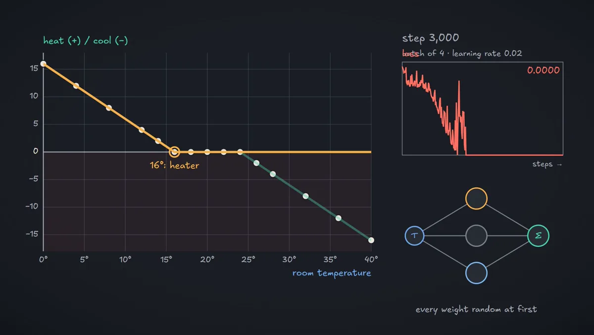
Each adjustable weight and bias then receives its own rate from that sweep. A training step moves the adjustable numbers together, after which the network makes another prediction. Real training often combines signals from a small group of examples before moving the numbers, then repeats with another group; a switched-off ReLU can block a route’s signal. The important distinction is that the target came from outside, while the internal corrections were calculated from the network’s own path to that target.
Try backpropagation
Follow one hidden answer to the end, then trace how the final mistake reaches it.
Predict before you reveal: if the output weight were 3, what would happen to an arriving message of −16?
Crossing that weight would make the message −16 × 3 = −48 at the hidden answer, provided the rest of that path is active. This is a sensitivity, not a direct instruction to subtract 48 from the neuron.
WHAT CHANGED? Earlier neurons receive a share of the final mistake, scaled along each route and added where routes meet.
Key concepts
- Backward pass
- The sweep from final loss toward earlier neurons that calculates how much each adjustable number affects that loss.
- Chain rule
- The reason sensitivities multiply along a path. When an output weight is ×2, the loss message to its input is also scaled by 2.
- Gradient accumulation
- Adding effects when one value influences the loss by several routes. In the active two-route example, −3 and −3 combine to −6.
- Batch
- A group of training examples whose signals are combined before an update. The lab traces one example so every step remains visible.
The compact version, once you have seen it
message through a weight = arriving message × that weightmessage at a fork = sum of messages from every route
After the backward sweep, every parameter has a gradient. A training step moves all of them together. The diagrams show one example; full training repeats on batches of examples.